Standartox - Standardizing Toxicity Data
An increasing number of chemicals such as pharmaceuticals, pesticides and synthetic hormones are in daily use all over the world. In the environment, chemicals can adversely affect populations and communities and in turn related ecosystem functions. To evaluate the risks from chemicals for ecosystems, data on their toxicity, which are typically produced in standardized ecotoxicological laboratory tests, is required. However, this kind of data is not always easy to retrieve in adequate formats. One could, in the case of pesticides find them in the Pesticide Property Data Base (PPDB), search the literature for these values or query the vast EPA ECOTOX knowledgebase. Yet, all of these methods or resources have their drawbacks.
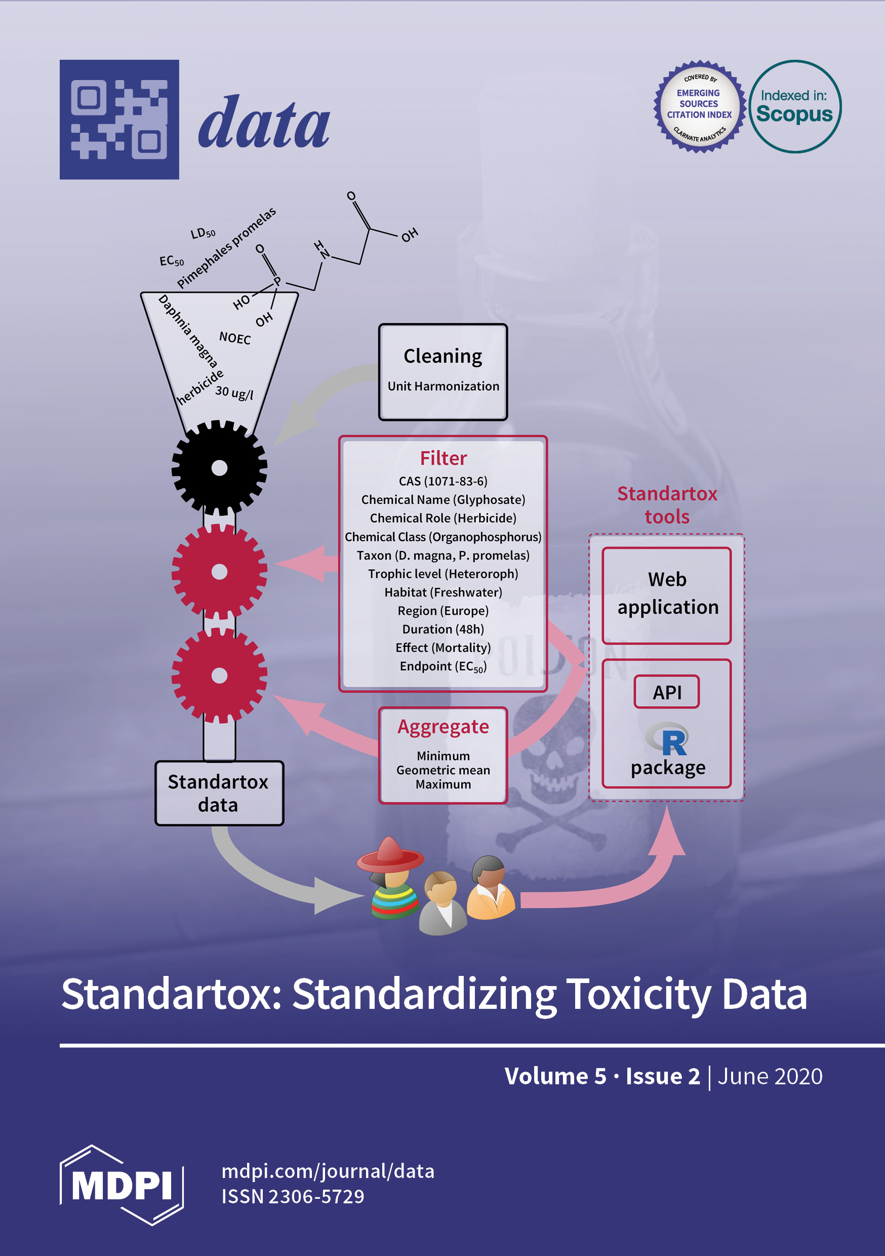
Here, Standartox steps onto the stage, by providing filter and aggregation methods for cleaned ecotoxicity data. Standartox is a tool and processing pipeline that continuously incorporates the ever-growing number of test results in an automated process workflow that ultimately leads to a single aggregated data point for a specific chemical-organism test combination, representing the toxicity of a chemical. These values can be used for the derivation of Toxic units (TU) or Species Sensitivity Distributions (SSD) For now Standartox relies solely on data of the quarterly updated EPA ECOTOX knowledgebase. This might be different in future releases. A paper about Standartox has recently been published at MDPI Data.
Standartox can be accessed through the web application http://standartox.uni-landau.de and the R package standartox, whereby the latter allows for more tailored queries and directly loading the data into R. The R package is built around a web service hosted at the university of Landau. This blog post will discuss, how to access Standartox via the R-package.
The R package
The Standartox R package mainly consists of the two functions stx_catalog()
and stx_query(). The former returns a catalog containing all possible parameters
and entries that can be used in the latter to query the actual data. Let’s start
with an example. Say, we are interested in the susceptibility of different
organisms towards Glyphosate.
Installation
First, we install and load the Standartox package together with other packages for data manipulation (data.table) and plotting (ggplot2). Since standartox is not yet on CRAN, we install it from GitHub.
# install.packages('remotes') # if remotes:: is not installed
# remotes::install_github('andschar/standartox') # package not yet on CRAN
require(standartox)
require(data.table)
require(ggplot2)
The catalog - stx_catalog()
Then, we directly use stx_catalog() to query the catalog of parameters that
can be used in the query function. We store the returned list object it in a
variable named catal. The parameters in catal are shown in the table below:
catal = stx_catalog()## Retrieving Standartox catalog..| parameter | example |
|---|---|
| casnr | 50000, 94815, 94826 |
| cname | 2439, 4, 3 |
| concentration_unit | ug/l, mg/kg, ppb |
| concentration_type | active ingredient, formulation, total |
| chemical_role | pesticide, herbicide, drug |
| chemical_class | amide, aromatic, organochlorine |
| taxa | species, genus, Fusarium oxysporum |
| trophic_lvl | heterotroph, autotroph |
| habitat | freshwater, terrestrial, marine |
| region | europe, america_north, america_south |
| ecotox_grp | invertebrate, plant, fish |
| duration | 24, 96 |
| effect | mortality, population, biochemistry |
| endpoint | NOEX, LOEX, XX50 |
| exposure | aquatic, environmental, diet |
| vers | 20191212 |
The query - stx_query()
Now, that we know what parameters can be set, we code the actual
query, thereby setting the casnr to 1071-83-6 (Glyphosate), choosing XX50 as
our endpoint and limiting the duration to a range from 24 to 120h,
amongst others. The query takes a little to complete (depending on the number
of chemicals provided).
l1 = stx_query(casnr = '1071-83-6', # Glyphosate
               endpoint = 'XX50', # contains EC50, LC50, ...
               concentration_unit = 'ug/l',
               duration = c(24, 120), # all in hours
               habitat = 'freshwater',
               concentration_type = 'active ingredient')
## Standartox query running..
## Parameters:
## casnr: 1071-83-6
## concentration_unit: ug/l
## concentration_type: active ingredient
## duration: 24, 120
## endpoint: XX50
## habitat: freshwaterstx_query() returns a list containing a filtered, a filtered_all
and the aggregated data set as well as a meta data set.
These are all data.tables (and data.frames) (Disclaimer: You might encounter
other list entries, which are currently work in progress and shouldn’t bother
you for now).
The filtered data set contains the most important information on the test result, including chemical names and identifiers (e.g. cas, inchikey), endpoint, effect and exposure groups as well as taxonomic information. Likewise, the converted and the original concentration and the duration together with the respective units are returned.
The filtered_all data set contains even more of this information, for example the EPA ECOTOX knowledgebase in-house identifiers and information on the reference, such as titles, authors and years.
The aggregated data set contains aggregated values, meaning the minimum, the geometric mean and the maximum for each chemical. Also, the taxa providing the minimum and maximum are included.
agg = l1$aggregated| cname | cas | min | tax_min | gmn | gmnsd | max | tax_max | n |
|---|---|---|---|---|---|---|---|---|
| glyphosate | 1071-83-6 | 5.3 | Gomphonema | 30500.84 | 1.949947 | 6209704 | Carassius auratus | 249 |
- The meta data set provides information on when, and from which version the data was queried, assuring reproducibility.
Plot the data
To get an overview of how the susceptibility of different taxa towards Glyphosate
varies, we plot the data, ordered from lowest to highest.
We choose to plot the data on the genus level. To calculate the geometric mean
for every genus and Glyphosate, we take the filtered data and and use a
non-exported function from within the standartox package
standartox:::gm_mean(x = ).
fil = l1$filtered # extract the filtered data.table
# aggregate over genera (data.table syntax)
fil_mn = fil[ ,
              .(gmn = standartox:::gm_mean(concentration)),
              by = .(tax_genus, ecotox_grp) ]
# build appropriate colors
col = c('deepskyblue4', 'yellowgreen', 'tomato4', 'darkgreen', 'goldenrod')
names(col) = unique(fil$ecotox_grp)
# plot
ggplot(fil) +
geom_point(aes(x = concentration,
y = reorder(tax_genus, -concentration),
col = ecotox_grp),
size = 2, pch = 1) +
geom_point(data = fil_mn,
aes(x = gmn,
y = tax_genus,
col = ecotox_grp),
size = 3) +
scale_x_log10(breaks = c(1e1, 1e2, 1e3, 1e4, 1e5, 1e6, 1e7),
labels = c(10, 100, 1000, 10000, 100000, 1e6, 1e7)) +
scale_color_manual(values = col,
name = 'Taxonomic\ngroup') +
labs(title = expression(Glyphosate~XX[50]~values), #'Glyphosate XX50',
x = 'Log10 Concentration (ug/l)') +
theme_bw() +
theme(axis.title.y = element_blank())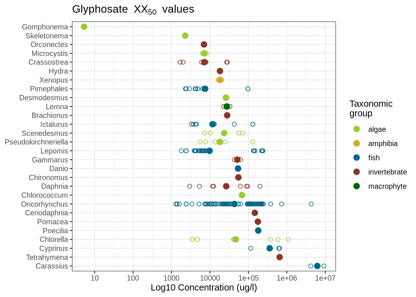
We observe that the two diatom genera Gomphonema and Skeletonema together with the crayfish genus Orconectes constitute the three most susceptible taxa. However, it appears that each of these taxa have only been tested once and we should probably have a look into the study whether we can trust the result or not. In contrast, the Oncorhynchus fish genus, for example is much better tested and exhibits a discrepancy ranging over several orders of magnitude, possibly also because of the many different species, including Rainbow trout and Pacific salmons comprised in the genus. Here it would be better to choose a specific Oncorhynchus species, related to the study area.
This is just a quick example on how to use Standartox. You can further
refine the query to your needs, by setting parameters, such as chemical_clas
chemical_role, trophic_lvl, region etc. Bear in mind though, this
data might not (yet) be complete.
Final Thoughts
Surely, such a project isn’t finished once the paper is published. New data is regularly included, data gaps need to be filled and errors, lurking most certainly somewhere in the depths of Standartox need to be corrected. Feel free to file an issue at the GitHub page if you find a bug or want to suggest a new feature. I also have plans to extend Standartox, which might be discussed in a future blog post. You also find a more detailed explanation of the R package at the project page.
By the way, if you need additional data for your chemicals, you most certainly can retrieve them with the help of the webchem R package, a project I’m also involved in.
Tech stack
To rebuild the Standartox database, all the necessary scripts can be found at the standartox-build GitHub page. Basically, the EPA ECOTOX knowledgebase is downloaded and built into a PostgreSQL database. There, several SQL and R processing scripts prepare the data. To build the web application Standartox relies on the shiny web framework and associated packages. The web service is built with the plumber R package. Throughout the project, the data.table package is used to guarantee fast processing. To allow fast data transmission, the filtered data is serialized using the fst R package before sending it to the users. Standartox’s code is located at the two GitHub repositories:
- standartox-build contains the processing scripts as well as web service and application definition files.
- standartox contains the code for the R-package.
Resources
- Blog post: https://andschar.github.io/2020/08/11/standartox
- Paper: https://www.mdpi.com/717852
- GDCH article (in German): https://www.gdch.de/fileadmin/downloads/Netzwerk_und_Strukturen/Fachgruppen/Umweltchemie_OEkotoxikologie/mblatt/2020/b2h120.pdf
- Blog post to build the EPA ECOTOX knowledebase locally: https://edild.github.io/localecotox